Abstract
The change in optical Earth observation since 2015 is usually described as sharper images and faster revisit. The description is accurate and it misses the more important development. The decade’s central achievement was not better cameras. It was cameras that could be used together. A set of correction methods, the clearest example being NASA’s Harmonized Landsat and Sentinel-2 product, now takes instruments built by different agencies, on different platforms, with different detectors, and makes their measurements interchangeable.
This paper follows that development from the open-data policy that began it, through the analysis-ready data standards that formalized it, to the geospatial foundation models trained on its output. It then follows the corrected product into orbit. In December 2025 the first geospatial foundation model to run in orbit met the same problem the ground correction was built to remove, and the size of that problem measures how much the ground pipeline had been doing.1
The argument is singular. Onboard optical inference inherits the work the ground correction leaves unfinished. A model trusts data from an unfamiliar sensor only if something reconciles the two, and in orbit the inputs that reconciliation depends on are mostly absent. There are two ways through. Which one prevails will shape the next decade. This is the optical companion to the SAR entry in this series.2
01 — The baseline that did not look like one
In June 2015 a satellite went up that did not look like a turning point. Sentinel-2A carried a wide-swath multispectral imager, thirteen spectral bands, and a 290-kilometer swath, and it asked nothing of the people who would eventually use it.3 The data was free. That was the change. Not the optics.
The optics were good and not remarkable. What Sentinel-2 did, and what Landsat had been doing in the open since 2008, was put a continuous, calibrated, public record of the land surface within reach of anyone with a connection. Imagery stopped being a line item. The cost that had shaped every prior workflow came off, and the workflows changed to match.
Two free archives are not one archive. Landsat 8 and Sentinel-2 saw the same ground with different detectors, different band definitions, different orbits, different overpass times, and different atmospheric conditions. Stack their observations without correction and the time series moves for reasons that have nothing to do with the land. Removing those instrument effects, so that what remains describes the surface, is the problem the rest of the decade organized itself around.
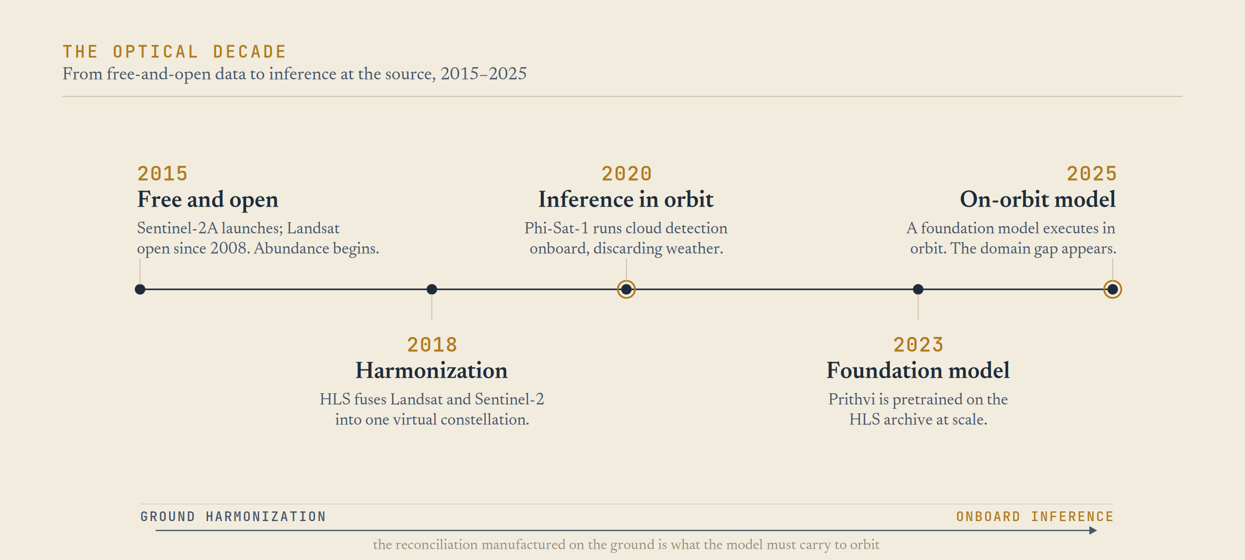
Figure 1 · The optical decade in one line. Free and open data (2015) makes the imagery available; HLS makes it comparable across sensors; the comparable record trains foundation models (Prithvi, 2023); the models move toward orbit (2025), where that correction is hardest to reproduce.
02 — Harmonized Landsat and Sentinel-2
The clearest example is the Harmonized Landsat and Sentinel-2 product. HLS is not a satellite. It launches nothing. It is a processing pipeline, run on the ground, that takes data from the Landsat 8 and 9 satellites and the Sentinel-2A, 2B, and 2C satellites and produces a single surface-reflectance product.4 The output is a virtual constellation: observations of the land roughly every 1.6 days at 30 meters, from instruments no one designed to work together.5
The pipeline runs a sequence of corrections, each one closing a specific difference between the two instruments.6
The harmonization pipeline, in plain terms.
| Step | What it reconciles |
|---|---|
| Atmospheric correction | Converts top-of-atmosphere signal to surface reflectance using a common algorithm (LaSRC) fed external atmospheric state, ozone and water vapor, from MODIS. The measurement becomes the land, not the air column. |
| Cloud and shadow masking | Flags pixels that are not ground, so a time series is not corrupted by weather read as change. |
| Co-registration and common gridding | Resamples both sensors onto the same Sentinel-2 tile system (MGRS), so a pixel from Landsat and a pixel from Sentinel-2 describe the same patch of ground. |
| View and illumination normalization | Adjusts for sun and view geometry (BRDF) so the same surface reads the same regardless of when and at what angle it was seen. |
| Spectral bandpass adjustment | Tunes the Sentinel-2 bands to match the Landsat spectral response, so the values agree across instruments. |
Output is gridded into Cloud Optimized GeoTIFFs on a common 30-meter basis. Each step removes a difference between the instruments. What remains describes the surface.
Every step in that table depends on something the satellite did not carry. The atmospheric correction needs ozone and water-vapor estimates from a separate spacecraft. The gridding needs a reference geometry. The angle normalization needs a model of how surfaces reflect at different sun and view angles. The bandpass adjustment needs a measured characterization of each sensor. None of this is in the raw image. All of it is added later, in a data center. The agreement between Landsat and Sentinel-2 that HLS delivers is produced on the ground, from inputs the satellite never had. That is the fact to keep in mind, because it returns when the work moves into orbit.
The product holds up. Independent comparison found the Landsat and Sentinel-2 outputs in close agreement across the spectral channels and very close on derived indices like the burn ratio, which is what licenses treating them as one stream.7 The record reaches back to the first Landsat 8 acquisitions in 2013 and the first Sentinel-2 acquisitions in 2015. HLS therefore did more than unify two sensors going forward. It produced a consistent optical record of the land surface a decade deep, at near-daily cadence. That record is what the foundation models would later train on.
03 — Analysis-ready data
HLS is one example of a broader pattern. Through the decade the burden of making imagery usable shifted from the user to the provider. The principle is called analysis-ready data: correct and standardize the imagery once, at the source, so that every downstream user does not repeat the work.
The Committee on Earth Observation Satellites formalized it. The CEOS-ARD definition sets the minimum a product must meet, calibrated radiometry, corrected geometry, documented per-pixel metadata, to support time-series analysis and cross-sensor use without each analyst rebuilding the correction stack by hand.8 The language is dry. The effect is not. Preprocessing that thousands of analysts used to perform separately is done once, by the provider.
Two technical standards made the principle operational. The Cloud Optimized GeoTIFF restructured the image file so a client can pull the few tiles it needs over HTTP without downloading the whole scene, which aligned imagery with the serverless, streaming architecture the rest of computing had already moved to. The SpatioTemporal Asset Catalog provided a common way to describe where and when an asset was collected, so software written once can discover imagery, SAR, point clouds, and data cubes from any provider that speaks the spec.9 COG answers how to read only what you need. STAC answers how to find it in the first place. Together they turned petabyte archives into something a script could browse.
Google Earth Engine had shown the model as early as 2010: convert the open archives to a cloud-optimized form, put the compute next to the data, and let users run analysis without moving the imagery. It produced work like planetary-scale forest-change mapping that would have been impractical under the download-everything model.10 The open standards generalized that approach so anyone could build on it.
These standards are the same idea as HLS, applied broadly. The imagery should arrive already corrected, already comparable across sensors and across time. Every later development in optical Earth observation assumes that work has already been done.
04 — The commercial parallel
The public agencies were not alone, and the commercial side arrived at the same principle from the opposite direction.
Planet’s approach was mass. Starting from a 28-satellite flock in 2014, the company scaled a constellation of shoebox-sized Doves to the point of imaging Earth’s entire landmass at roughly three-meter resolution every day, a cadence no government system matches.11 Daily revisit changes the question you can ask. A weekly record lets you confirm something you already suspect. A daily record lets you notice changes you were not looking for.
Planet also built in interoperability on purpose. Its SuperDoves are designed to register against public imagery like Sentinel-2, and the products are calibrated for sensor and atmospheric differences for use in time series.12 A commercial operator, answering to customers rather than to a standards committee, reached the same conclusion the agencies had: corrected, comparable imagery is worth more than raw pixels, and the correction is part of the product.
Planet’s high-resolution Pelican satellites, deploying through 2025, carry NVIDIA Jetson modules and process imagery onboard before downlink, cutting the time from tasking to delivered result to hours rather than days.13 The same pressure that pushed correction onto the ground is now pushing computation into orbit. Collection was never the constraint. The constraint is the distance between collection and a usable answer.
05 — Harmonized data as training data
A consistent, decade-deep, daily optical record is more than a convenience for analysts. It is a training set.
NASA and IBM built Prithvi for this, a geospatial foundation model pretrained on the HLS archive. The first generation, released in August 2023, was the largest open geospatial AI model of its moment. The second, Prithvi-EO-2.0, released in late 2024 at up to 600 million parameters, was trained on 4.2 million global time-series samples drawn directly from HLS at 30-meter resolution, across six surface-reflectance bands, and benchmarked to outperform a field of competing models.14
The sequence matters. A pipeline built to make Landsat and Sentinel-2 agree produced a record consistent enough to train a foundation model on. The correction came first. The model depended on it. Prithvi learns to recognize floods, burn scars, croplands, and coastlines from data whose consistency across sensors and across years was produced on the ground by the steps in that table. Without that correction, the model would have learned the instruments’ quirks as if they were properties of the land.
The model was possible because the data had already been made consistent. The correction came first, on the ground, years before anyone trained on it.
The first essay in this series tracked this shift for onboard AI in general. It shows up most sharply in optical, because the optical archive is the most consistent and the strongest models were trained on it. The models are capable and the compute is already moving to orbit. The next step is to run the model on the satellite, on the data as it is collected.
06 — Inference moves to the source
This is already happening, and it has been from the start. The first optical model to run in orbit shows both the appeal and the limit.
Its job was the most natural one in optical imaging: discard clouds. Clouds cover roughly two-thirds of the Earth at any moment, so a satellite that downlinks everything spends most of its bandwidth sending weather to the ground to be thrown away. ESA’s Phi-Sat-1, launched in September 2020, ran a convolutional network called CloudScout on an Intel Movidius Myriad 2 accelerator. It identified scenes above a cloud threshold and discarded them before downlink, saving about a third of the bandwidth.15 The decision moved onto the satellite. Only the usable images were sent down.
How CloudScout was trained is worth noting. The team did not have enough imagery from its own new sensor, so they trained the network on Sentinel-2 data pre-processed to match that sensor’s response.16 The first optical model to fly already faced the cross-sensor problem, and the fix was to build a matched training set on the ground, simulating the in-orbit sensor before launch. The same correction work that HLS does was present at the start of onboard optical AI, done quietly inside the training data.
Five years later the ambition grew from a single narrow classifier to a general one. In December 2025, researchers demonstrated the first on-orbit execution of a geospatial foundation model, compressing Prithvi-EO-2.0 by a factor of sixteen, from roughly 1.2 gigabytes to 73 megabytes, through knowledge distillation, and running it on flight-representative hardware, with live inference performed on the IMAGIN-e payload aboard the International Space Station.17 It is one model serving many tasks, running where the data is collected. This is the arrangement the first essay anticipated, now reaching optical, the data type with the deepest corrected archive behind it.
The demonstration also produced the result that matters most here. When the team moved the HLS-and-Sentinel-trained model to a different sensor, the Kanyini mission’s imager, performance fell hard. Cloud-detection accuracy dropped by roughly 48 percent and the false-positive rate rose by more than half, driven by the mismatch in spatial resolution, in radiometric calibration, and in spectral response between the sensor the model learned on and the sensor it now faced.18 The researchers call this the domain gap. It is the cross-sensor problem from Section 02, met in a place where the usual fix is not available.
The domain gap in orbit is the cross-sensor problem of Section 02, encountered without the tools that solve it. HLS closes that gap on the ground using MODIS atmospherics, reference geometry, BRDF models, and bandpass characterization. A satellite running a model in orbit carries none of that.
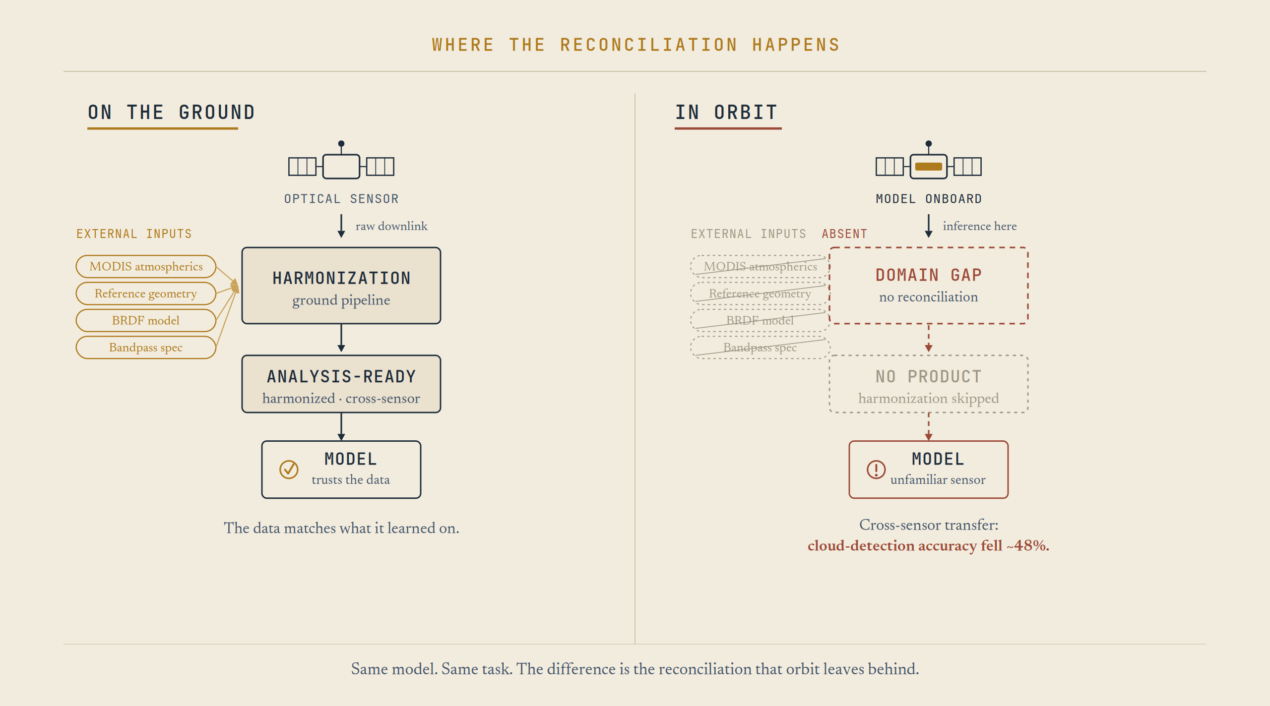
Figure 2 · Where the correction happens. The processing that makes optical models reliable is assembled on the ground, from inputs the satellite does not carry. Running inference onboard moves it away from those inputs, which is what produces the domain gap.
This is the part the resolution and revisit numbers never capture. The foundation models were made possible by correction performed on the ground, using inputs the satellite does not have. Running the model in orbit moves it away from those inputs. The model reaches the point of collection, which is the point where the correction is hardest to perform. The first essay described downlink as the bottleneck that pushes processing upward. On the optical side there is a further problem: the corrected data that made the model reliable was built on the ground, in the place the model is now leaving.
07 — The unfinished work
The domain gap is not a defect in one experiment. It is the basic condition of onboard optical inference, and it defines two paths, which together describe the next decade of the field.
The first path is to perform the correction onboard. Give the satellite enough calibration and sensor characterization to bring its own data into the form the model expects before the model runs. This is HLS in miniature, done within a power and memory budget measured in watts and megabytes instead of a data center. It is hard, because some of what HLS relies on, a second satellite’s atmospheric measurements, a global reference geometry, is not available to a single spacecraft working in real time. A lighter version, domain adaptation, was demonstrated in the on-orbit work: retrain the model’s task heads on a small amount of data from the new sensor. It recovers much of the lost accuracy, but it has to be redone for each sensor and is not a general fix.19
The second path inverts the problem. Rather than forcing every sensor’s data into one corrected form before inference, design the inference, and especially its output, to hold up without that correction. Build the model and the product it emits to be sensor-agnostic, so that what comes off the satellite is a portable, comparable result regardless of which instrument produced the pixels behind it. On this path the differentiator is not the detection algorithm, which is increasingly a commodity foundation model. It is the output data model: a representation stable enough that a flood map from one sensor and a flood map from another mean the same thing, and can be combined, without a ground-side correction step standing between collection and use.
Which path prevails is an open question with real stakes. It determines whether the value in onboard Earth observation goes to whoever owns the most sensors, or to whoever sets the output standard that lets different sensors work together. The SAR entry in this series closed on the orbital compute buildout, the accelerators going up to handle radar’s data rates.20 The optical case adds a layer. The compute is necessary and it is arriving. The open questions are what it runs on and whether its output is portable across sensors, which is the same correction problem the decade was built around, now placed where it is hardest to solve.
The last decade’s work was getting two sensors on the ground to agree. The next decade’s work is getting a model in orbit to handle a sensor it was not trained on. It is the same problem moved to a harder place, where the corrections that solved it before are no longer at hand.
§ § §
Methodology & source tiers
This paper synthesizes open technical and primary-source material under a three-tier scheme. Tier 1 (primary / peer-reviewed / official): NASA, USGS, and ESA mission and product documentation (HLS product pages and User Guide, Sentinel-2 mission documentation), the CEOS-ARD specification, and peer-reviewed and preprint literature including the Phi-Sat-1 / CloudScout work (Giuffrida et al., 2021), the Prithvi-EO-2.0 model and paper (2024), and the first on-orbit geospatial foundation model demonstration (Du et al., arXiv:2512.01181, 2025). Tier 2 (specialist / institutional): IBM Research and NASA Science communications on Prithvi, Clark University Center for Geospatial Analytics, eoPortal mission profiles, Ubotica Technologies, and the cloud-native geospatial standards bodies (COG, STAC). Tier 3 (press / secondary): trade and encyclopedic compilations used only for non-load-bearing context (constellation histories, launch chronologies).
Two cautions are load-bearing. First, the claim is about a structural inheritance, that onboard optical inference faces the cross-sensor correction problem harmonization solves on the ground, and it rests on a single demonstrated instance of the domain gap (the December 2025 on-orbit work) generalized cautiously; the gap’s size is task- and sensor-dependent, and the same study showed some tasks degrade far less or even improve. Second, capability claims are bounded to what the sources support: onboard optical inference, including a compressed foundation model, is demonstrated and flown, but general-purpose onboard inference across arbitrary sensors without adaptation is not yet a fielded capability. The two-paths framing in Section 07 is analysis, not forecast.
-
Andrew Du, Roberto Del Prete, Alejandro Mousist, et al., “First On-Orbit Demonstration of a Geospatial Foundation Model,” arXiv:2512.01181 (1 December 2025). The work reports the first onboard execution of a geospatial foundation model and the domain gap encountered when transferring it across sensors. ↩
-
BlueLens Analytics, “Inference at the Source: A Literature Review of Onboard AI in Earth Observation, 2019–2026,” BLA-TR-2026-02. The present paper is the optical companion to that broader, SAR-leaning review. ↩
-
ESA, “Introducing Sentinel-2” and “Copernicus: Sentinel-2” (eoPortal). Sentinel-2A launched 23 June 2015 carrying a 13-band multispectral imager with a 290-kilometer swath; Sentinel-2B followed in 2017 and Sentinel-2C in 2024. The US Landsat archive was opened for free public access in 2008, establishing the open-data precedent the Copernicus program extended. ↩
-
NASA Earthdata, “Harmonized Landsat and Sentinel-2 (HLS)”; NASA GSFC HLS project pages. Two products are generated, L30 from Landsat 8/9 OLI and S30 from Sentinel-2 MSI, radiometrically harmonized and gridded to a common 30-meter basis. ↩
-
NASA Earthdata HLSS30 and HLSL30 v2.0 catalog entries. The combined virtual constellation enables global land observation roughly every 1.6 days at 30 meters. ↩
-
NASA Earthdata and HLS Product User Guide (v1.5 provisional, LP DAAC). The pipeline applies atmospheric correction (a C implementation of the Land Surface Reflectance Code, LaSRC, using MODIS-derived ozone and water vapor), cloud and cloud-shadow masking, spatial co-registration and common MGRS gridding (cubic-convolution resampling to reconcile the Landsat and Sentinel-2 tiling origins), view and illumination (BRDF) normalization to a nadir-adjusted reflectance (NBAR), and spectral bandpass adjustment of S30 to match the Landsat 8 spectral response. Output layers are written as Cloud Optimized GeoTIFFs. ↩
-
Cross-comparison of HLS L30 and S30 against established Landsat-8 surface-reflectance measures reported high agreement across spectral channels and very high agreement on the Normalized Burn Ratio, with low relative root-mean-square differences (per the spectral-correspondence assessment published in Science of Remote Sensing, 2021). ↩
-
Committee on Earth Observation Satellites, “CEOS Analysis Ready Data” (ceos.org/ard). CEOS-ARD specifies threshold and goal requirements for metadata, radiometric and atmospheric correction, and geometric correction, defined as the minimum level required to support time-series analysis and data interoperability. ↩
-
Cloud Optimized GeoTIFF specification (cogeo.org, now an OGC standard) and the SpatioTemporal Asset Catalog specification (stacspec.org). COG enables efficient partial reads of imagery over HTTP; STAC provides a common, extensible language for describing and discovering spatiotemporal assets across providers. ↩
-
On Google Earth Engine (2010) as the first large-scale adoption of cloud-optimized open archives co-located with compute, and the research it enabled including global forest-change mapping, see the analysis-ready-data overview in GeoConnexion (2020). ↩
-
Planet Labs constellation documentation and eoPortal “Planet — Flock Imaging Constellation.” From the 28-satellite Flock 1 (2014), the PlanetScope / SuperDove fleet scaled to image Earth’s entire landmass at roughly 3-meter resolution on a near-daily basis across eight spectral bands. ↩
-
Planet, “Planet Monitoring” and SuperDove product material; eoPortal Planet profile. SuperDoves are described as interoperable with publicly available imagery such as Sentinel-2, with products pre-processed and calibrated for sensor differences and atmospheric conditions for temporal analysis. ↩
-
Planet Labs and eoPortal “Planet Pelican.” The Pelican constellation, deploying through 2025, carries NVIDIA Jetson modules for on-orbit edge computing to process data before downlink; the system is engineered with inter-satellite links and high downlink rates for end-to-end tasking-to-delivery latency on the order of hours. ↩
-
Daniela Szwarcman, Sujit Roy, Paolo Fraccaro, et al., “Prithvi-EO-2.0: A Versatile Multi-Temporal Foundation Model for Earth Observation Applications,” arXiv:2412.02732 (December 2024); IBM Research and NASA Science communications. Prithvi-EO-1.0 (August 2023) was the largest open geospatial AI model at release; Prithvi-EO-2.0 (up to 600M parameters) was trained on 4.2 million global time-series samples from NASA’s HLS archive at 30-meter resolution across six surface-reflectance bands and benchmarked on GEO-Bench against competing models. ↩
-
Gianmarco Giuffrida, Luca Fanucci, Gabriele Meoni, et al., “The Φ-Sat-1 Mission: The First On-Board Deep Neural Network Demonstrator for Satellite Earth Observation,” IEEE Transactions on Geoscience and Remote Sensing (2021); Ubotica Technologies mission communications. Phi-Sat-1 (launched September 2020 on the FSSCat mission) ran the CloudScout CNN on an Intel Movidius Myriad 2 accelerator to identify and discard scenes above a ~70 percent cloud threshold before downlink, with reported bandwidth savings on the order of 30 percent. Clouds obscure roughly two-thirds of Earth’s surface at any moment, which is what makes onboard cloud screening the natural first optical edge application. ↩
-
G. Giuffrida et al. (2021); “CloudScout: A Deep Neural Network for On-Board Cloud Detection on Hyperspectral Images,” Remote Sensing 12(14):2205 (2020). CloudScout was trained and tested on a dataset extracted from Sentinel-2 imagery, pre-processed to emulate the HyperScout-2 hyperspectral sensor, because insufficient data from the novel target sensor was available, an explicit ground-side reconciliation of the training distribution to the in-orbit sensor. ↩
-
Du et al., arXiv:2512.01181 (2025). Prithvi-EO-2.0-300M was compressed roughly 16× (about 1.2 GB to 73 MB) via dual-MAE knowledge distillation while retaining downstream task performance, and executed on flight-representative hardware (Myriad-2 class accelerators and the IMAGIN-e compute module), with onboard inference validated aboard the International Space Station. ↩
-
Du et al., arXiv:2512.01181 (2025). Transferring the source-trained model to the Kanyini mission sensor produced a substantial domain gap: tile-level cloud-detection accuracy dropped by roughly 48 percent and the false-positive rate rose by more than half, attributed to spatial-resolution mismatch (Sentinel-2’s 10–20 m versus Kanyini’s ~75 m) compounded by radiometric and spectral differences. The same study found the gap is task-dependent, with flood segmentation showing modest gains. ↩
-
Du et al., arXiv:2512.01181 (2025). Domain adaptation, retraining lightweight task heads on a fraction of target-sensor labels while keeping the foundation backbone frozen, recovered much of the lost performance and improved data efficiency, but is applied per target sensor rather than as a general reconciliation. ↩
-
BlueLens Analytics, “Inference at the Source,” BLA-TR-2026-02, on the orbital compute buildout (orbital data centers and flight-class accelerators) driven by the data rates of modern sensors, SAR in particular. ↩