I’ve been running ESA SNAP (European Space Agency’s Sentinel Application Platform) as my primary SAR preprocessing engine for some time now. Not as an academic exercise but as the actual workhorse of production pipelines I deliver to clients. What I want to write about here is the gap between what SNAP is documented to do and what it takes to make it run reliably at operational scale. That gap is real, and it costs people time they don’t have.
This is the third post in a series on the actual mechanics of geospatial intelligence work. The first covered why LLMs are structurally well-suited for GIS workflow design and where autonomous execution falls apart. The second, “Independent by Design,” detailed why I primarily use open-source tools in my workflows, avoiding proprietary software traps and saving significant amounts of money. This one gets more specific: a concrete SAR preprocessing chain using SNAP, driven by Python, pulling from the Copernicus Data Space Ecosystem, and built to run repeatedly with a minimal amount of supervision. Supervision is critical, however, and I do not recommend full automation at this time with agentic AIs.
Why SNAP, and Why It’s Worth the Friction
There is a reasonable argument that you should skip SNAP entirely and go straight to pyroSAR or snappy or one of the newer Python-native SAR tools. I’ve made that argument myself. But SNAP is still the reference implementation for Sentinel-1 processing, and its Graph Builder architecture [the GPT graph system] gives you something that Python-native tools don’t: a fully reproducible, serializable preprocessing workflow that you can version-control, audit, and hand off to an analyst who has never written a line of code.
A .xml GFT graph is not glamorous. But when a client needs to reproduce your processing chain six months later in a different environment, a graph file is more trustworthy than a Python script with three layers of abstraction and a requirements.txt that’s already drifting.
The friction is real though. SNAP’s headless mode [invoking gpt from the command line] is where the interesting failure modes live. That’s where we’re going.
The Collection Problem First
Before SNAP touches anything, you need data. ESA’s Copernicus Data Space Ecosystem replaced SciHub in late 2023, and if you’re still pointing at SciHub endpoints you’ve already lost. CDSE uses an OData API with OAuth2 token-based auth, which is a meaningful change from SciHub’s basic auth over REST.
The practical issue is token management at scale. OAuth2 tokens expire. If you’re running an overnight batch against a 30-scene AOI mosaic and your token expires at scene 12, your download stalls silently unless you’ve built refresh logic into the collector. This isn’t in the CDSE quickstart. It’s something you discover the hard way.
Here’s an example script of the type of pattern I frequently use:
class CDSECollector:
    def __init__(self, client_id, client_secret):
        self.token_url = "https://identity.dataspace.copernicus.eu/auth/realms/CDSE/..."
        self.client_id = client_id
        self.client_secret = client_secret
        self._token = None
        self._token_expiry = 0

    def _get_token(self):
        if time.time() < self._token_expiry - 60:
            return self._token
        resp = requests.post(self.token_url, data={
            "grant_type": "client_credentials",
            "client_id": self.client_id,
            "client_secret": self.client_secret
        })
        resp.raise_for_status()
        payload = resp.json()
        self._token = payload["access_token"]
        self._token_expiry = time.time() + payload["expires_in"]
        return self._token
That sixty-second buffer before expiry has saved batch jobs more times than I can count. The get_token call goes into every download request, not just the first one.
The Preprocessing Chain
Once you have scenes on disk, the preprocessing chain for Sentinel-1 GRD is well-established. The question is whether you’re running it through the GUI, through snappy, or through headless GPT. For production, the answer is headless GPT with a version-controlled graph file.
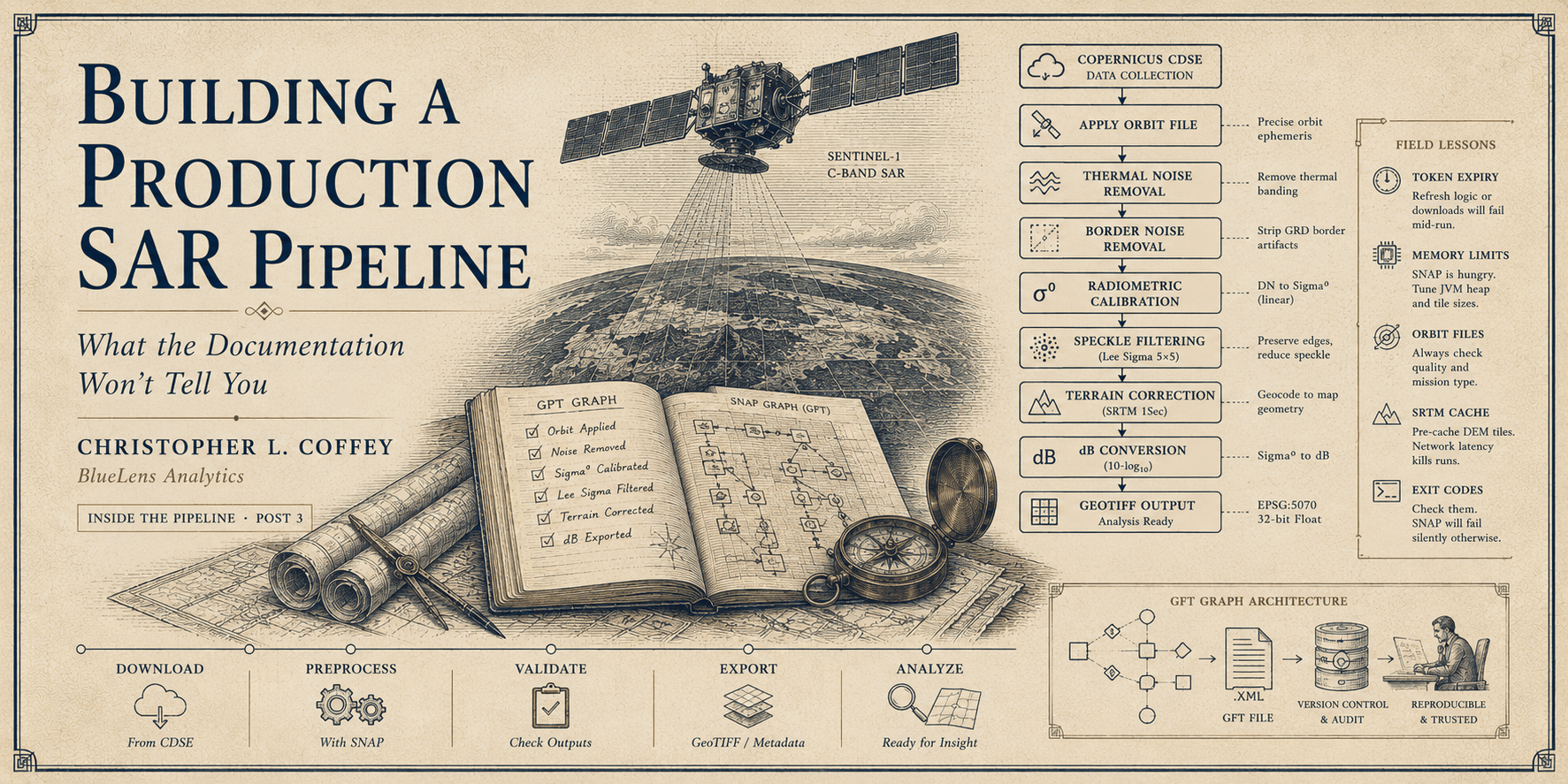
The full chain [from raw GRD to analysis-ready GeoTIFF] runs in this order:
-
Apply Orbit File: corrects orbital state vectors using the precise orbit ephemeris. Skip this and your terrain correction geometry will be slightly wrong. Slightly wrong compounds.
-
Thermal Noise Removal: removes thermal noise banding artifacts from the GRD product. Matters most at range edges. Not optional if you’re doing any kind of intensity-based analysis.
-
Border Noise Removal: strips the invalid data strips at scene borders introduced during SLC-to-GRD conversion.
-
Radiometric Calibration: converts digital numbers to sigma₀ in linear units. For most change detection work, Sigma₀ is correct.
-
Speckle Filtering: Lee Sigma at a 5×5 kernel is my standard for urban and mixed-use monitoring. It preserves edges better than a boxcar and doesn’t over-smooth the point scatterers that are diagnostic in infrastructure monitoring. It is critical that you vary the kernel density value for different environments when applying SPECKLE filters! This is the critical difference between zero returns, useless returns, or a single artifact render of the entire image scene.
-
Range-Doppler Terrain Correction: projects slant-range geometry into a map-projected coordinate system. I tend to use SRTM 1Sec HGT at 10m output spacing. If your AOI has terrain relief greater than ~500m, elevation model quality starts mattering. You will quickly learn the limitations of your system processing power.
-
Linear to dB: log conversion before export. dB values are more interpretable, more normally distributed, and more stable for threshold-based change detection. This is absolutely critical and non-negotiable in SAR applications of any kind.
-
Write: GeoTIFF, EPSG:4326, dual band (VV, VH). For starters anyway. GeoTIFF is the format. I will write another blog explaining why.
In a GPT graph, that’s eight connected operators. The graph file is clean XML. You can look at it in a text editor. You can diff it in git. When something changes in your output and you need to know why, the graph is the ground truth.
Where SNAP’s Headless Mode Will Surprise You
Running gpt your_graph.xml -Pinput=/path/to/scene.zip -Poutput=/path/to/output.tif sounds simple. It mostly is, until:
- Memory. SNAP’s default JVM heap allocation is too small for large GRD scenes at 10m spacing. Set -J-Xmx16G in the gpt.vmoptions file. The error messages when you hit the heap ceiling are not always clear about what’s happening.
- Orbit files. Apply Orbit File downloads auxiliary data on first use. In an air-gapped or restricted-network environment, it fails silently and produces slightly miscorrected output. Pre-stage the orbit files and point SNAP at a local AuxData directory via snap.auxdata.root, somewhere like ~/.snap/etc/snap.properties
- SRTM downloads. Same issue with terrain correction. Pre-stage the tiles before you run in a restricted environment.
- Parallel execution. gpt is not thread-safe at the process level in all configurations. Spawn each invocation as a separate OS process with its own temp directory.
- Exit codes. GPT exits 0 even on soft failures in some versions. Check that your output file exists and has nonzero size. Don’t trust the exit code alone.
Wiring It Together
The pattern I run in production is a thin Python orchestrator that handles the CDSE download, file staging, and subprocess dispatch to GPT. Here’s a sample:
import subprocess
from pathlib import Path

def run_snap_graph(graph_path, input_path, output_path,
                   snap_gpt="/opt/snap/bin/gpt"):
    cmd = [
        snap_gpt,
        str(graph_path),
        f"-Pinput={input_path}",
        f"-Poutput={output_path}",
        "-J-Xmx16G",
        "-q", "4"
    ]
    result = subprocess.run(cmd, capture_output=True,
                            text=True, timeout=3600)
    if result.returncode != 0:
        raise RuntimeError(f"GPT failed:\n{result.stderr}")

    out = Path(output_path)
    if not out.exists() or out.stat().st_size == 0:
        raise RuntimeError(f"GPT exited 0 but output missing: {output_path}")

    return out
That output size check has caught real failures that the exit code didn’t. Add it. Also add a hash of the input file to your processing log; when you’re debugging why a specific scene processed differently from the rest, knowing the exact input file state matters.
The Part Where This Connects to Something Larger
Everything above is infrastructure. The reason it’s worth getting right is that what runs downstream of this preprocessing chain is where actual intelligence value lives.
Calibrated, terrain-corrected, dual-polarization GeoTIFFs in consistent coordinate space are the optimal input to coherence analysis, backscatter change detection, and log-ratio differencing for activity indicators. That’s fun party conversation right there y’all!
If the preprocessing chain is inconsistent [such as different orbit correction states; different terrain model vintages; different filter parameters between acquisitions] the change signal you’re trying to detect is contaminated by processing variance. That noise is invisible unless you’ve tracked your pipeline state carefully.
I’ve seen analysts spend weeks trying to understand anomalous change signals that turned out to be an inconsistent speckle filter applied to a subset of the time series. The anomaly was in the processing, not the scene. Forgotten or hidden terrain model coordinate system projection corrections will make your life miserable.
Reproducibility isn’t a nice-to-have in SAR change detection. It’s a prerequisite for the analysis being meaningful.
What’s Next
The next post in this series covers change detection proper: log-ratio differencing, coherence-based detection, and scene-adaptive thresholding using Otsu’s method on the processed outputs this pipeline produces. That’s where the interesting analytical problems start and the point where the data pipeline begins to become something you can trust. A bit. Proper application of Otsu parameters can greatly reduce speckle filtering and other incredibly resource intensive computational processes in the stack, and I find it to be of great use in limiting token burn and GPU churn.
Chris Coffey is Senior AI Architect at BlueLens Analytics, a geospatial intelligence consultancy based in the North Carolina Sandhills. BlueLens Analytics supports prime contractors, defense tech firms, and federal agencies with SAR processing pipelines, change detection systems, and AI-assisted geospatial analysis.